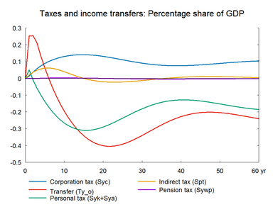
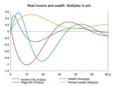
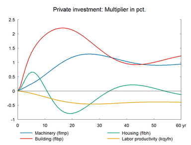
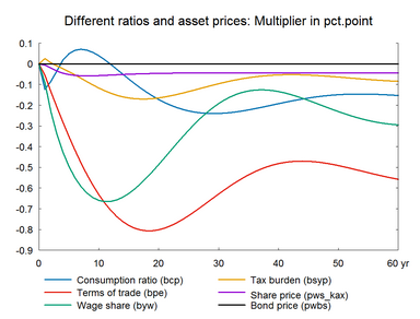
The focus now shifts to supply side shocks. Section 10-14 demonstrate the properties of ADAM to supply side shocks. Labor input in ADAM's production function is defined in terms of efficiency corrected labor hours, i.e. as a product of three elements: labor productivity, annual working hours per employed and employment. A change in any of these three components changes the labor input, and the experiments in section 10 - 12 present a shock to each of these three elements. In all cases, production increases in the medium and long run. In this section, labor supply is increased by increasing the number of workers. As in the previous experiments, each of the following six experiments (section 10 - 15) also include a sub-section where each multiplier exercise is repeated with a balanced public budget.
As mentioned earlier, the export relations in the current model version include supply effects. Expansion in labor force and productivity boosts production capacity making it possible to produce different varieties of a product. This leads to higher foreign demand shifting the demand curve outward and making it possible to sell higher exports without reducing prices. The positive response of exports to domestic output growth amplifies the effect on output and employment, because exports can expand without a need for declining terms of trade.
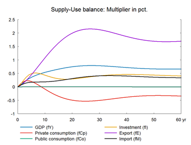
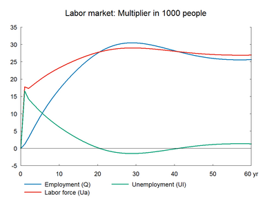
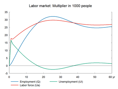
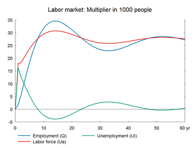
Here we consider the effect of a permanent increase in the number of people in the work force caused by a reduction of 1 percent of total employment in the number of people outside the labor force not receiving transfers. The work force increases approximately by 27000 people. (See experiment)
Table 10a. The effect of a permanent increase in labor supply
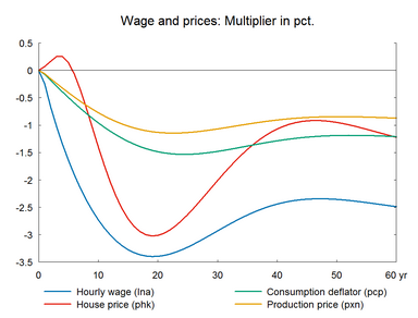
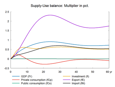
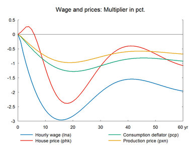
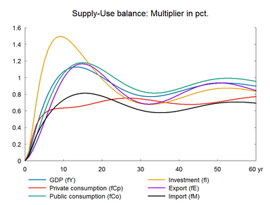
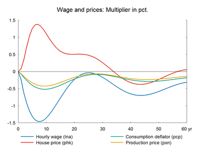
The increased labor supply is not automatically employed at once as there is no demand side response, so unemployment increases. The higher unemployment reduces the growth of wages and prices. The decline in prices relative to the baseline improves competitiveness, as a result production and exports increase and gradually pull the extra labor force into employment. Employment increases until the additional labor force is employed and the rate of unemployment is back at its structural level.
The positive effect on employment, the negative effect on wages and the positive effect on exports is permanent. Private consumption rises in the short run as the unemployed people receive unemployment benefits and other social benefits. The long term impact on private consumption is negative due to the negative real wage effect.▼ Real wage effect arises because wages increase/decrease more than the general price levels due to the deadweight from the non-responding exogenous import prices. This creates a positive/negative real wage effect, terms of trade and real disposable income and private consumption increase/decrease permanently. When domestic demand falls the export needs to increase even more for the extra supply of workers to be soaked up in the economy. For this to happend, terms of trade need to be even better. Thus, wage will have to decrease more.
Overall, there is a positive effect on production in the long run because of the permanent increase in employment. There is also a permanent change in the relative prices of production factors, as labor becomes relatively cheaper compared to the partly imported capital. This implies a substitution effect.▼ A substitution effect arises when a change in the relative prices of factors induces producers to use more of a relatively cheaper factor and less of a relatively more expensive factor. Consequently, the substitution of labor for capital making production more labor intensive and reducing labor productivity. The substitution effect offsets part of the increase in production.
The wage share falls permanently, i.e. the distribution of income changes permanently in favor of capital. Wage relative to user cost falls in the long run because investment prices fall less than wages due to the deadweight from import prices.
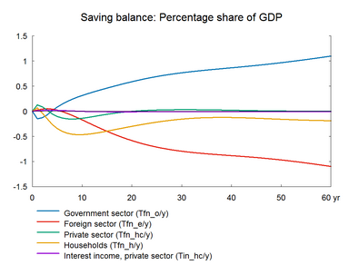
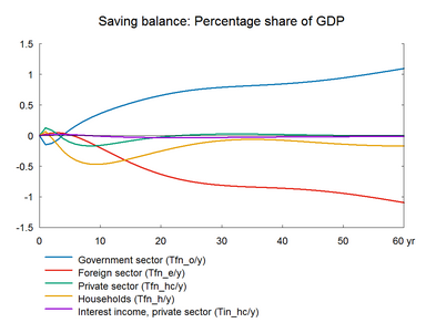
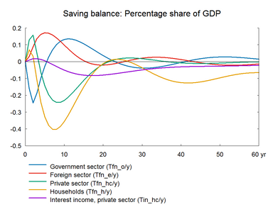
There is a significant positive effect on public budget in the long term, because the nominal fall in revenues is less than the nominal fall in expenditures. Transfer payments and public wage-expenses decline as hourly wages fall. Other public expenditures also fall as prices fall. On the revenue side, taxes on personal income fall when hourly wages fall. But the number of tax payers increases and this offsets some of the fall in tax revenue.
Figure 10a. The effect of a permanent increase in labor supply
|
||||||||||||||||||||||||||||||||||||||||||||||||||||||||||||||||||||||||||||||||||||||||||||||||||||||||||||||||||||||||||||||||||||||||||||||||||||||||||||||||||||||||||||||||||||||||||||||||||||||||||||||||||||||||||||||||||||||||||||||||||||||||||||||||||||||||||||||||||||||||||||||||||||||||||||||||||||||||||||||||||||
Increasing the labor supply has a permanent positive effect on domestic output; and it is likely that the market shares of danish exporter will rise. Table 10b presents the effect of a permanent increase in labor supply accompanied by supply effects in foreign trade. As in section A, the number of people outside the labor force not receiving transfers is reduced by 1 percent of total employment - approximately 27.000 people and, in contrast to section A, export performance are improved by an elasticity of 0.7 relative to GVA (gross value added).(See experiment)
Table 10b. The effect of a permanent increase in labor supply, with supply effects
Figure 10b. The effect of a permanent increase in labor supply, with supply effects
|
||||||||||||||||||||||||||||||||||||||||||||||||||||||||||||||||||||||||||||||||||||||||||||||||||||||||||||||||||||||||||||||||||||||||||||||||||||||||||||||||||||||||||||||||||||||||||||||||||||||||||||||||||||||||||||||||||||||||||||||||||||||||||||||||||||||||||||||||||||||||||||||||||||||||||||||||||||||||||||||||||||
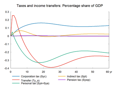
Increasing the labor supply has a permanent positive effect on the public budget balance. The additional public savings can be used to increase spending or to reduce tax rates in order to create expansionary effects in the economy. Table 10c presents the effect of a permanent increase in labor supply accompanied by a permanent decrease in income tax rates. As in section A and B, the number of people outside the labor force not receiving transfers is reduced by 1 percent of total employment - approximately 27.000 people and, in contrast to section A and B, central government income tax rates are reduced permanently by 6.16 percent (e.g. from 15 to 14.08 per cent) to balance the public budget in the long run.(See experiment)
Table 10c. The effect of a permanent increase in labor supply, balanced budget
The lower income tax rates reduce government revenues and public savings fall. In the short run, the negative effect on the public budget dominates, but in the long term, public budget and debt constitute the same ratios of GDP as in the baseline.
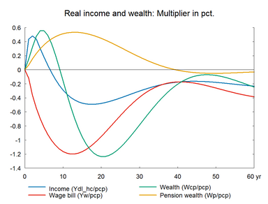
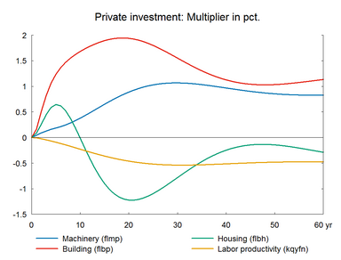
The higher labor supply is not immediately employed, so unemployment increases in the short run. The higher unemployment exerts a downward pressure on wages and prices which improves competitiveness. This makes exports stimulate production and employment. The expansionary effect is reinforced by higher private consumption, which peaks after five years. The higher consumption reflects that the lower income tax rates have increased disposable income. The stronger domestic demand makes unemployment fall more sharply than in section-A. Employment keeps increasing until the additional labor force is employed and the rate of unemployment has returned to its baseline. The higher production increases the capital stock and investments permanently. Imports also increase permanently to meet the higher domestic demand.
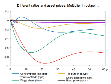
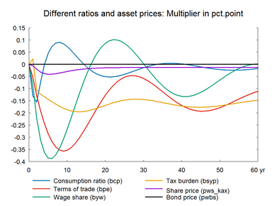
When the government budget is unchanged as a share of GDP, the balance of payment is also unchanged in the long run as indicated in table 10b. Moreover, in this balanced-budget experiment net exports remain fairly unchanged implying that the volume change in net exports is balanced by the price change. This balancing of nominal exports and imports is illustrated in figure 10a, where the percentage increase in real exports minus the percentage increase in real imports, cf. first diagram on the left hand side, is equal to the percentage deterioration in the terms of trade, cf. last diagram on the right hand side.
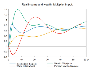
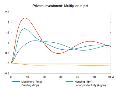
In the long run, the need for lower wages to boost competitiveness will moderate the increase in real income and private consumption. The initial consumption boom raises the demand for dwellings, housing investment and house price increase, and the higher housing wealth has a certain feed-back effect on private consumption. Moreover, the short-run expansion of the housing capital is stronger than the long run effect. The excess supply of houses created in the medium run reduces house prices and the housing investment is adjusted downwards before the housing market reaches its equilibrium.
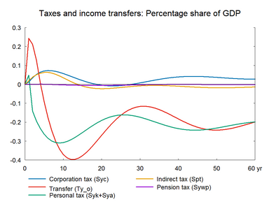
Figure 10c. The effect of a permanent increase in labor supply, balanced budget
|
||||||||||||||||||||||||||||||||||||||||||||||||||||||||||||||||||||||||||||||||||||||||||||||||||||||||||||||||||||||||||||||||||||||||||||||||||||||||||||||||||||||||||||||||||||||||||||||||||||||||||||||||||||||||||||||||||||||||||||||||||||||||||||||||||||||||||||||||||||||||||||||||||||||||||||||||||||||||||||||||||||
This section illustrates the effect of introducing a budget constraint to the labor supply shock in section A and B. Spending the supply-driven improvement in public finances on fiscal easing makes employment increase faster, and the long-run need for higher exports and improved competitiveness is also lower in section C. In section A and B, the additional labor supply was used to boosted public savings and net exports. In section C, it is primarily used to increase domestic consumption. Making the public sector spend its additional revenues resembles an introduction of Say’s law.
In a closed economy, spending the full-structural-employment GDP on consumption and investment would be enough to secure full structural employment. However, in an open economy a share of domestic demand will be met by higher imports, and exports will have to increase accordingly. Consequently, we still get an export increase in section C, but as we have seen, the export increase is smaller than in section A and especially in section B. In real terms, the long-run increase of exports in ADAM will always match full-structural-employment GDP plus imports minus domestic demand. And in section C, the increase of exports will also match the increase of imports in nominal terms, because the constant public budget plus the private consumption function makes the impact on domestic demand match the impact on GDP in nominal terms.
